Dive into Machine Learning Live Projects with Styrish AI
Introduction
Let’s start our fantastic journey with machine learning lessons online. Machine Learning is a field of artificial intelligence that emphasizes on the development of algorithms and statistical models that enable computer systems to perform tasks without explicit programming. It involves the use of data to train a model, which can then make predictions, decisions, or identify patterns. The process of machine learning involves the steps like, collecting and pre-processing the data, training data model, testing it using validation dataset, calculating loss and optimizing it till the best results are achieved.
Machine learning encompasses various types, with the primary categories being Supervised Learning, Unsupervised Learning, and Reinforcement Learning. Each type involves distinct methodologies and applications, providing a diverse landscape of learning approaches within the field.
Supervised Learning
Supervised learning is a type of machine learning where the algorithm is trained on a labelled dataset, which means the input data is matched with corresponding output labels. In simple words, supervised learning is like teaching a computer by showing it examples and telling it the correct answers. Imagine you have pictures of cats and dogs, and you tell the computer which ones are cats and which ones are dogs. The computer learns from these examples and tries to figure out the differences between cats and dogs. During this learning process, the computer adjusts itself to get better at recognizing cats and dogs. It’s a bit like training a pet – you show it what’s right and wrong, and it learns over time. The goal is for the computer to make accurate predictions on new pictures it hasn’t seen before, just like your pet would recognize a new animal it has never encountered.
Classification (Supervised Learning)
Classification, a type of supervised learning, involves training an algorithm to categorize data based on specific output labels or classes. This encompasses diverse classification types, such as Binary Classification, where the algorithm decides between two classes like determining whether an email is “spam” or “not spam.” Additionally, Multi-Class Classification handles tasks like categorizing data into nuanced classes such as “good” “better” or “best”, or, identifying images of distinct animal species.
Various machine learning algorithms prove beneficial for classification tasks, some of which are outlined below. To illustrate these algorithms, we’ll use a widely used Python library called scikit-learn.
Support Vector Machines (SVM)
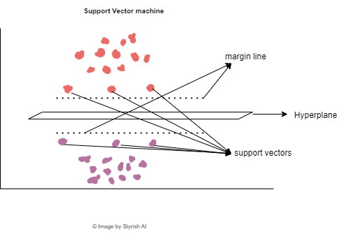
The Support Vector Machine (SVM) is a supervised machine learning algorithm used for both classification and regression tasks. Its functioning revolves around identifying the optimal hyperplane in a higher-dimensional space to effectively separate data points belonging to different classes, ensuring an optimal and maximized margin between them. SVM takes a set of input data points, each belonging to various classes, and maps the data to higher dimensional space. Further, it finds a hyperplane that best separates the data points of different classes. A hyperplane is a decision boundary that maximizes the margin, which is the distance between the closest data points (support vectors) of the two classes.
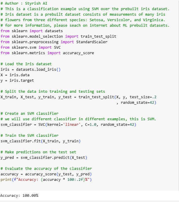
Once the data has been separated, data points are said to be classified. Example of SVM using scikit-learn is below. Here the prebuilt dataset for iris flowers has been used, which is available in scikit-learn library. The data was split into train and test with the ratio of 80:20, where 20% percent of data is used for validation after the training is done on 80% of data. (Test train split with 80/20 is standard practice. However, that can be altered based on the need).
K-Nearest Neighbours (KNN)
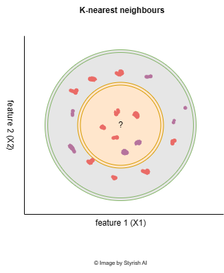
K-Nearest Neighbors (KNN) is a machine learning algorithm that identifies the nearest neighbors for an unknown data point, which is currently under examination. The algorithm operates on the principle that in a scattered distribution of data points on a plane, the unknown data point is likely to be closely related to its nearest neighbors, as points with similarity tend to be located in close proximity to each other.
The Euclidean distance formula is often used to determine the distance between the datapoints. For example, if there are two datapoints having feature as age, with value 34 and 36, their similarity will be calculated based on the Euclidean distance between those two points, which will be as below:
Consider two datapoints X and Y having two features such as, age and income. X (age=36, income=100), Y (age=32, income=150). Euclidean distance between datapoints in two-dimensional space will be:
General formula of Euclidean distance is as below:
One of the challenging aspects of using KNN is determining the appropriate value for K. The selection of K is critical as it signifies the number of neighbors to be considered around the unknown datapoint during the prediction process. The algorithm assigns the predicted class based on the majority class among the nearest neighbors within the specified range of K. If K is set too low, such as 1, it results in an overly specific model, considering only the single nearest data point, which may lead to incorrect predictions. Conversely, setting K to an extremely high value creates an overly generalized model that may not capture the nuances of the data.
To identify the optimal value for K, it is advisable to start with a small K, train the model, and evaluate its accuracy. Subsequently, fine-tune the value of K to achieve the highest accuracy with minimal loss. This iterative process helps find the most suitable and effective value of K for the given dataset and problem.
Example of KNN using scikit-learn library is given below:

Logistic regression
Irrespective to its name, Logistic regression is used in classification, not regression. Logistic regression is used primarily in classification problems, where your data is binary. In other words, Logistic regression is used primarily in classification problems, where can be classified as 0/1, True/False, Yes/No etc. Logistic regression can also be used for cases, where you need probability of your prediction. For example, the probability of buying a certain product by customer.
Logistic regression uses the Logistic function (Sigmoid) to calculate the probability. Logistic function always has the output between 0 to 1. 0 means 0% and 1 means 100%. Logistic function can be defined as below:
Here, θTX (Theta transpose X) is a linear combination of the input features and their weights, which can be given as:
To make predictions, a decision boundary is set. For binary classification, if the predicted probability P(Y=1) is greater than a chosen threshold (typically 0.5), the input is classified as belonging to the positive class (1); otherwise, it is classified as belonging to the negative class (0).
Example of Logistic regression using scikit learn library is given below:

Decision Trees
Decision trees are also one of the most popular machine learning algorithms, which is used for both classification and regression tasks. They are a type of supervised learning algorithm that makes decisions by recursively splitting the dataset into subsets based on the most significant attribute at each step. The result is a tree-like structure where each internal node represents a decision based on a specific attribute, each branch represents the outcome of that decision, and each leaf node represents the final decision or prediction.
The topmost node in the tree is called root node, which represents the entire dataset. Nodes that represent decisions based on specific features or attributes are called internal nodes, and the terminal nodes that provide the final output or decision are called leaf nodes.
At each internal node, the algorithm selects the best attribute to split the data based on a specific criterion. some of them includes:
Gini impurity (used in classification), that calculates the probability of incorrectly classifying a chosen element. The lower the value of Gini impurity, the better the split.
Entropy (used in classification), that measures the amount of information disorder or uncertainty. This should be progressively decreased while going down through the tree. This reduction in entropy signifies an improvement in the homogeneity of the subsets at each node, resulting in a more informative and decisive tree structure.
Mean squared error (used in regression), which is helpful to predict the accuracy of decision tree model. As per its name, MSE measures the average squared difference between the actual and predicted values.

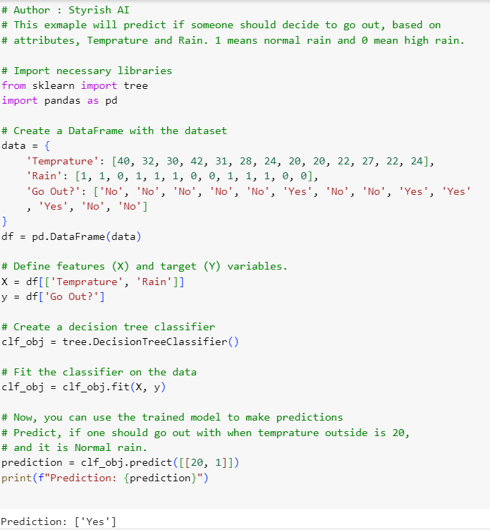
Example of decision tree using scikit-learn library is given below:
Regression (Supervised Learning)
Regression is a technique in supervised machine learning employed to forecast continuous values by leveraging other variables present in a dataset. The variables within the dataset used to anticipate the output value are termed independent variables (designated as X). Conversely, the forecasted value, or output, falls under dependent variables (designated as Y). An illustrative use case of regression involves predicting a house price based on its features, including floor area, location, and provided amenities. The regression process diverges from classification, where the model predicts a continuous value instead of predicting a class, as explored in previous sections on classification.
There are various machine learning algorithms available for regression. One of the widely used technique is Linear regression. Let’s understand that.
Linear regression
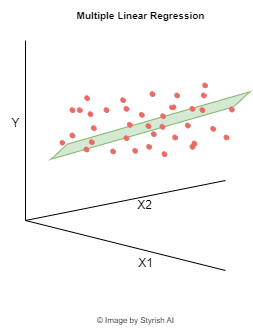
Linear regression is a regression algorithm that identifies the linear relationship between the dependent variable (Y) and independent variable(s) (X). The primary objective of linear regression is to discover the optimal linear equation that accurately captures this relationship. In the context of simple linear regression, where there is only one dependent variable and one independent variable, the relationship can be expressed as a straight-line equation. In contrast, for multiple linear regression, where there are multiple independent variables influencing a single dependent variable, the relationship is articulated using an equation of a hyperplane, extending the concept to a multidimensional space.

The objective of this algorithm is to determine the most suitable values for the coefficient ‘m’ and ‘c’ in a manner that minimizes the calculated loss between the predicted and actual values of the dependent variable ‘y’. This loss, commonly computed in regression tasks, is predominantly assessed using the Mean Squared Error (MSE) function. The MSE is derived by determining the average of the squared differences between the actual and predicted values of the dependent variable. For more information about MSE, please refer What are Optimizers and Loss Functions?
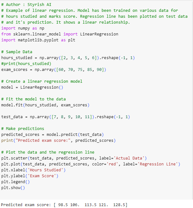
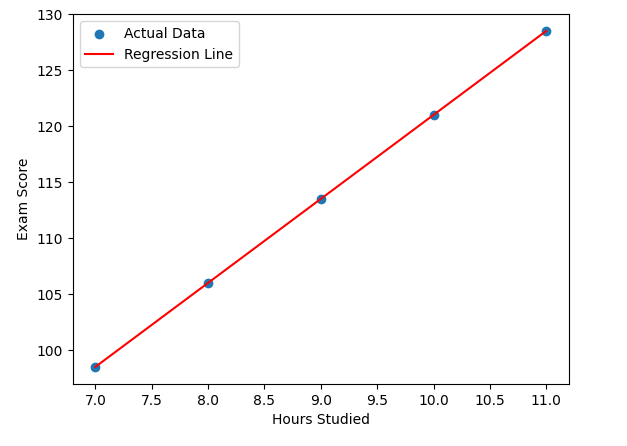
Example of Linear regression using scikit-learn library is given below.
Unsupervised Learning
Unsupervised learning is a type of machine learning where the algorithm is trained on a dataset without explicit supervision, meaning that the algorithm is not provided with labeled output data. In other words, the algorithm tries to learn the patterns and relationships within the data without being explicitly told what to look for or how to interpret the input. One of the use cases of unsupervised learning is grouping the customers based on their purchasing behaviors.
One of the widely used algorithm used in unsupervised learning is K-means clustering. Let’s understand that.
K-means clustering
It is a partitioning clustering, which divides the data into non-overlapping subsets (clusters), without any cluster-internal structure. Clustering means grouping the data based on their characteristics. Examples within the clusters are very similar, and very different across the cluster. The similarity between the datapoints is mostly calculated by Euclidean distance formula, and the lower distance examples are kept together in a single group. Euclidean distance has been explained in the section (K-nearest Neighbours) above. Apart from this, similarity can also be calculated using other mechanisms like cosine similarity, Jaccard similarity, Manhattan distance etc.
